

Thermo-Hydraulic Simulation of Piping Systems

The DSHplus Piping Systems Library offers a sophisticated computational model that accurately describes the temperature-dependent behavior of both liquid and gaseous fluids as they move through a complex pipe network. This model not only considers heat exchange with the environment, but also accounts for pressure- and temperature-dependent fluid properties, ensuring a realistic and precise representation of thermal-fluid dynamics.
By solving the thermo-hydraulic governing equations, the simulation predicts transient pressure drops, fluid temperatures, and flow rates at any point in the system. This allows engineers to gain valuable insights into how a system reacts to changing thermal and hydraulic conditions, making it an essential tool for performance evaluation and optimization.
Applications in Engineering and Industry
Thermo-hydraulic simulations are widely used in the design and optimization of piping systems across various industries. Typical applications include:
- Cooling circuits in industrial machinery and power plants, where efficient heat dissipation is critical.
- Chemical processing plants, where maintaining precise thermal conditions affects reaction efficiency and safety.
- Power generation systems, such as steam and gas turbine cycles, where optimizing heat exchange improves energy output.
- Heating, ventilation, and air conditioning (HVAC) systems, where balancing temperature distribution ensures energy efficiency and comfort.
With DSHplus, engineers can simulate, analyze, and refine the thermal and hydraulic performance of piping networks, leading to improved system efficiency, reduced energy consumption, and enhanced reliability. Whether for research, industrial applications, or engineering design, DSHplus provides a powerful solution for mastering complex thermo-hydraulic challenges.
Overview of the Thermo-Hydraulic Functions
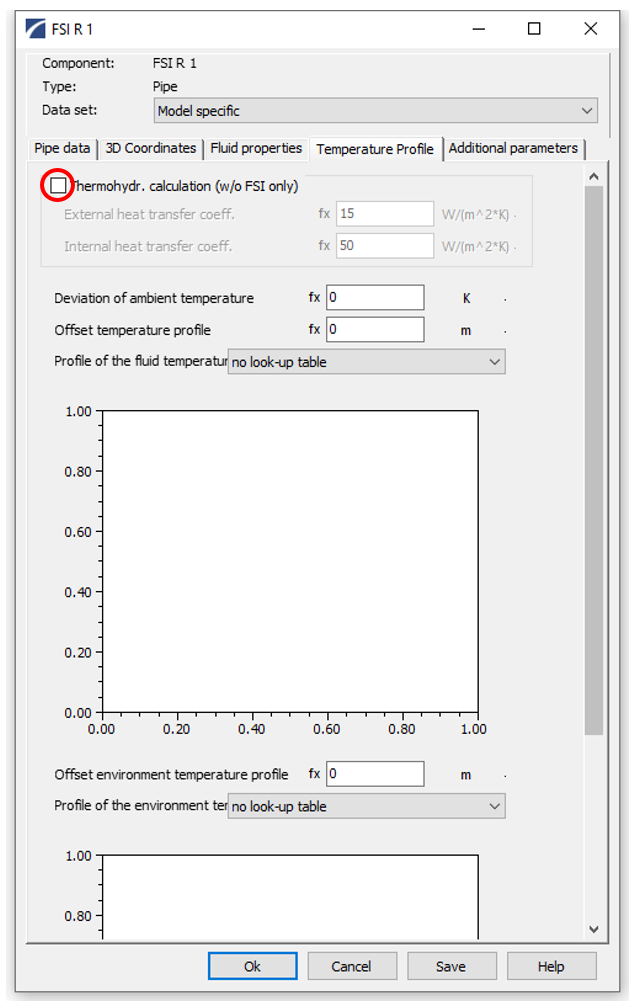
By activating the option “Thermohydraulic calculation”, the default equation system consisting of the momentum and continuity equation is extended by the energy equation.
The heat flow can either be imposed directly via the input "Heat Flow" or calculated based on the heat transfer coefficients under consideration of the ambient temperature. The option "Profile of the ambient temperature" allows the user to specify a distribution of the ambient temperature.
The heat transfer between the fluid and the pipe wall and between the pipe wall and the environment are described through the parameters "Internal heat transfer coefficient" and "External heat transfer coefficient".
The mathematical model covers the following phenomena:
- Heat transfer between the fluid and the environment (description via thermal transmittance)
- Dissipative heating due to pressure drop
- Increase of pressure in closed systems due to increase of temperature
- The transport of energy with the flow (convective transport)
The mathematical model currently does not take the following phenomena into account:
- Increase in heat transfer due to higher flow velocities
- Pressure, flow rate or temperature-dependent heat transfer coefficients
- Thermal conduction in axial direction
- Thermal capacity of the pipe wall
Heat Transfer Between the Fluid and the Environment
Required parameters:
- Characteristic map for environmental temperature $T_{Env}$ distribution or single parameter defining the deviation from the environmental temperature provided in the environment component
- Internal & external heat transfer coefficients
- Thermal conductivity of pipe material $k_W$
- Wall thickness
Based on these parameters, the thermal transmittance $U$ between the liquid and the environment is calculated:
$$U = \frac{1}{\frac{1}{\alpha_i}+\frac{r_i}{k_W}ln(\frac{r_a}{r_i})+\frac{r_i}{\alpha_a r_a}}$$
The heat flux $\dot{q}^"$ (per unit area of the inner pipe surface) exchanged between liquid and environment is then given by:
$$\dot{q}^" = U(T_F-T_{Env})$$

Application Example of Thermo-Hydraulic Simulation
- The system of three identical parallel pipes is initially at rest and pre-charged to 20 bar. The oil temperature is 293 K. The environmental temperature is set to 363 K.
- Within the first 0.5 s, a flow rate of 10 l/min is established.
- Intention of the test is to show the three different possibilities to consider heat transfer through the pipe wall in a thermohydraulic simulation.
Heat transfer with fixed heat transfer coefficients
The first pipe uses the heat transfer coefficients as parametrized in the dialog. Due to the higher environmental temperature, there is a net heat flow from the environment through the pipe wall to the oil. Thus, the oil temperature at both pipe ends (blue and grey temperature curve in the upper figure) increases at the start of the simulation. With beginning oil flow after 1 s, “fresh” oil enters the pipe from the left-hand side. Consequently, the oil temperature at the left-hand side (grey temperature curve) of the pipe drops to tank temperature level. The outlet temperature (blue curve) at the right-hand side of the pipe approaches a steady level when the first “slice” of fresh oil (which has entered the left side of the pipe at the onset of oil flow) has travelled through the entire pipe.
Heat transfer with time-variant heat transfer coefficients
On the second pipe the input for the external heat transfer coefficient overrules the parameterized value and the externally provided value is used for calculation. For the first second of the simulation, the external heat transfer coefficient is set to zero. If viscous heating due to fluid friction is negligible, the fluid temperature remains unchanged.
After 2 seconds, the external heat transfer coefficient is set to the standard value (red curve in the lower figure). Due to the higher environmental temperature, now there is a positive heat flow through the pipe wall into the oil and the red temperature curve in the upper figure increases. The temperature reaches the same steady-state level as for the standard pipe after the first “slice” of fresh oil (which has entered the left side of the pipe after the heat transfer coefficient was set) has travelled through the entire pipe.
Heat transfer with imposed time-variant heat flow
The third pipe uses the input for the external heat flow - the heat transfer coefficients are ignored. Positive (heating) and negative (cooling) heat flows are allowed. A negative heat flow has a cooling effect on the fluid temperature.
For the first 4 seconds of the simulation, the external heat flow is set to zero. After 4 seconds, the external heat flow is set to the value depicted in the green curve of the lower figure. The value is calculated by multiplying the thermal transmittance U with the inner pipe surface and the log. average temperature difference between oil and environment. Again, the temperature reaches a steady level when the first “slice” of fresh oil that has entered the left side of the pipe (after the heat flow has been switched on) has travelled through the entire pipe.

