Pressure Losses With Incompressible Pipe Flow

In piping systems, unavoidable pressure losses occur, significantly impacting the performance and efficiency of hydraulic and pneumatic systems. These losses arise due to friction along pipe walls and local flow resistances caused by bends, contractions, valves, or fittings. In energy-efficient systems, a precise analysis of these losses is crucial, as they directly affect the energy demand of pumps and compressors as well as the overall system efficiency.

In incompressible flow, where the fluid density remains constant, velocity-dependent pressure losses are influenced by several factors:

Pipe length and diameter affect flow velocity and frictional losses.
Surface roughness increases turbulence, amplifying energy losses.
Flow velocity and Reynolds number determine whether the flow is laminar or turbulent, which in turn affects frictional losses.

To analyze and optimize such flow effects, the DSHplus Piping Systems Library provides a powerful simulation solution. This library includes a detailed representation of velocity-dependent influences on pressure loss within piping components, enabling realistic 1D-CFD simulations. This allows engineers to not only model piping systems with high accuracy but also optimize them for energy efficiency and optimal operation.

By using DSHplus, engineers can perform a comprehensive design and optimization of piping systems, reduce energy losses, and enhance the efficient operation of fluid power applications.

Theoretical Background

With an incompressible pipe flow (Pipe radius $r_a$) is the pressure loss per unit length $\Delta p/\Delta z$ in balance with the wall shear stress ${\tau}$ exerted by the flow on the pipe wall:

$$\frac{\Delta p}{\Delta z} = \frac{2}{r_a}\tau$$The wall shear stress of Newtonian fluids (e.g. hydraulic oils, water, air) can be calculated from the slope of the velocity profile $u(r)$ at the wall ($r=ra$):
$$\tau = -\eta \frac{\partial u}{\partial r}\bigg\vert_{r=r_a}$$
where $u$ is the variable axial velocity component of the pipe flow over the radial coordinate $r$ ($0 \le r \le r_a$) is the variable axial velocity component of the pipe flow and $\eta$ is the dynamic viscosity of the fluid.

If the velocity profile u(r) is known as a function of the volume flow Q or as a function of the cross-section averaged flow velocity u¯=Q/A, then a correlation between pressure drop and volume flow or between pressure drop and cross-section averaged velocity can be established.

Pressure Loss in Steady Laminar Flow Through a Pipe

For steady laminar flows through circular pipes, the Navier-Stokes equation can be solved exactly. This allows the resulting velocity profile $u(r)$ to be specified as a function of the cross-section-averaged flow velocity $\bar{u}$: $$u(r) = 2\bar{u}\left[1-\left(\frac{r}{r_a}\right)^2\right]$$ For the wall shear stress $\tau$, this results in: $$\tau = -\ eta \frac{\partial u}{\partial r}\bigg\vert_{r=r_a} = \frac{4\eta}{r_a}\bar{u}$$ This results in the following for the pressure loss: $$\frac{\Delta p}{\Delta z} = \frac{8\eta}{r_a^2}\bar{u}$$ This relationship is known as HAGEN and POISEUILLE's law. If you want to use the volume flow $Q$ instead of the cross-sectional average flow velocity, you can write: $$\frac{\Delta p}{\Delta z} = \frac{8\eta}{\pi r_a^4}Q = \frac{128\eta}{\pi D^4}Q$$ Here, $D$ denotes the diameter of the pipe.

Analogous to Ohm's law in electrical engineering, Hagen-Poiseuille's law can also be represented using hydraulic resistance $R_H$: $$\Delta p = R_H Q$$ The hydraulic resistance of a pipe with a length $l$ is given by: $$R_H = \frac{128\eta l}{\pi D^4}$$

Pressure Loss in Steady Turbulent Pipe Flow

If the Reynolds number $Re$ of the pipe flow exceeds a critical value $Re_{crit} \approx 2300$, the flow transitions from laminar to turbulent. Since no exact solution for the Navier-Stokes equation for turbulent flow is known to date, the velocity profile for this type of flow must be determined experimentally. However, if one is only interested in the relationship between the pressure loss per unit length $\Delta p/\Delta z$ and the cross-section-averaged flow velocity $\bar{u}$, it is more practical to measure this directly. The results of such measurements are usually represented in the literature by the so-called pipe friction factor $\lambda$. This indicates the pressure loss relative to the dynamic pressure $\rho\bar{u}^2 /2$ and the relative pipe length $\Delta z/D$: $$\lambda = \frac{2D}{\rho \bar{u}^2} \frac{\Delta p}{\Delta z}$$ If $\lambda$ is known, the pressure loss can be calculated as follows: $$\frac{\Delta p}{\Delta z} = \frac{\lambda}{D}\frac{\rho}{2}\bar{u}^2$$ This relationship is known as the law of DARCY and WEISSBACH. If you want to calculate using the volume flow instead of the cross-sectional average flow velocity, you can write: $$\frac{\Delta p}{\Delta z} = \frac{\lambda}{D}\frac{\rho}{2}\frac{Q^2}{A^2}$$

The pipe friction factor depends on the Reynolds number $Re$; in the case of hydraulically rough pipes, there is also a dependence on the relative roughness $\varepsilon/D$ of the pipe wall. For hydraulically smooth pipes with Reynolds numbers $2300 < Re < 10^5$, the formula from BLASIUS applies:

$$\lambda = \frac{0.3164}{\sqrt[4]{Re}}$$

Pressure Loss in Unsteady Laminar Pipe Flow

In unsteady flow, the velocity profile differs from that in steady flow. As the velocity distribution changes, so does the slope of the velocity profile at the pipe wall, which leads to a change in the wall shear stress compared to steady flow. The change in wall shear stress results in a different pressure loss in unsteady flow. In 1966, ZIELKE [1] succeeded in expressing the instantaneous wall shear stresses and thus the pressure loss as a function of past changes in the volume flow. According to this, the total pressure loss in unsteady laminar flow is the sum of the steady-state pressure loss and the unsteady pressure loss:

$$\frac{\Delta p}{\Delta z} = \frac{128\eta}{\pi D^4} Q(t) + \frac{64\eta}{\pi D^4} \int_{0}^{t} \! W_d(t-t_1)\frac{\partial Q(t_1)}{\partial t} \, \mathrm{d}t_1 $$

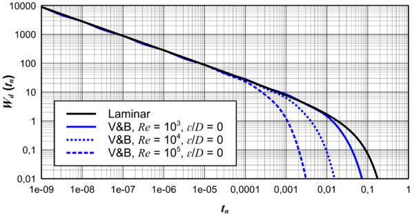
Here, $W_d$ denotes the transient (“dynamic”) portion of the weighting function $W$, which weights past volume flow changes in terms of their significance for the current pressure loss.

Pressure Loss in Unsteady Turbulent Pipe Flow

Even in the case of unsteady turbulent pipe flow, the unsteady pressure loss is calculated using a convolution integral. However, in this case, the dynamic weighting function $W_d$ also depends on the Reynolds number and the wall roughness $\varepsilon/D$ relative to the pipe diameter, as is the case with steady flow. The following applies: $$\frac{\Delta p}{\Delta z} = \frac{\lambda}{D}\frac{\rho}{2}\frac{Q^2(t)}{A^2} + \frac{64\eta}{\pi D^4} \int_{0}^{t} \! W_d(t-t_1)\frac{\partial Q(t_1)} {\partial t} \, \mathrm{d}t_1 $$ The weighting function $W_d$ is calculated in DSHplus according to a paper by VARDY and BROWN [2].

The dynamic weighting functions $W_d$ for laminar and turbulent flows are shown in the following figure over the normalized time $t_n = t\nu/D^2$.

Literatur

[1] ZIELKE, Werner. Frequency dependent friction in transient pipe flow. 1966. Doktorarbeit. University of Michigan.

[2] VARDY, Alan E.; BROWN, Jim M. Approximation of turbulent wall shear stresses in highly transient pipe flows. Journal of Hydraulic Engineering, 2007, 133. Jg., Nr. 11, S. 1219-1228.